Knowledge
Two Flatness Zones, Two Opposite Verdicts on the Same Part
"Half this part passes and half of it fails" is the flatness result that generates the longest meetings. Manufacturing suspects the machine or the way it was placed. Quality argues that one failure means the part fails. Both sides then spend considerable time arguing over a single number without first settling a more basic question: are these two flatness values even describing the same thing?
This article uses real inspection data to settle that question. The data is unremarkable, which is exactly why it demonstrates the point so cleanly.
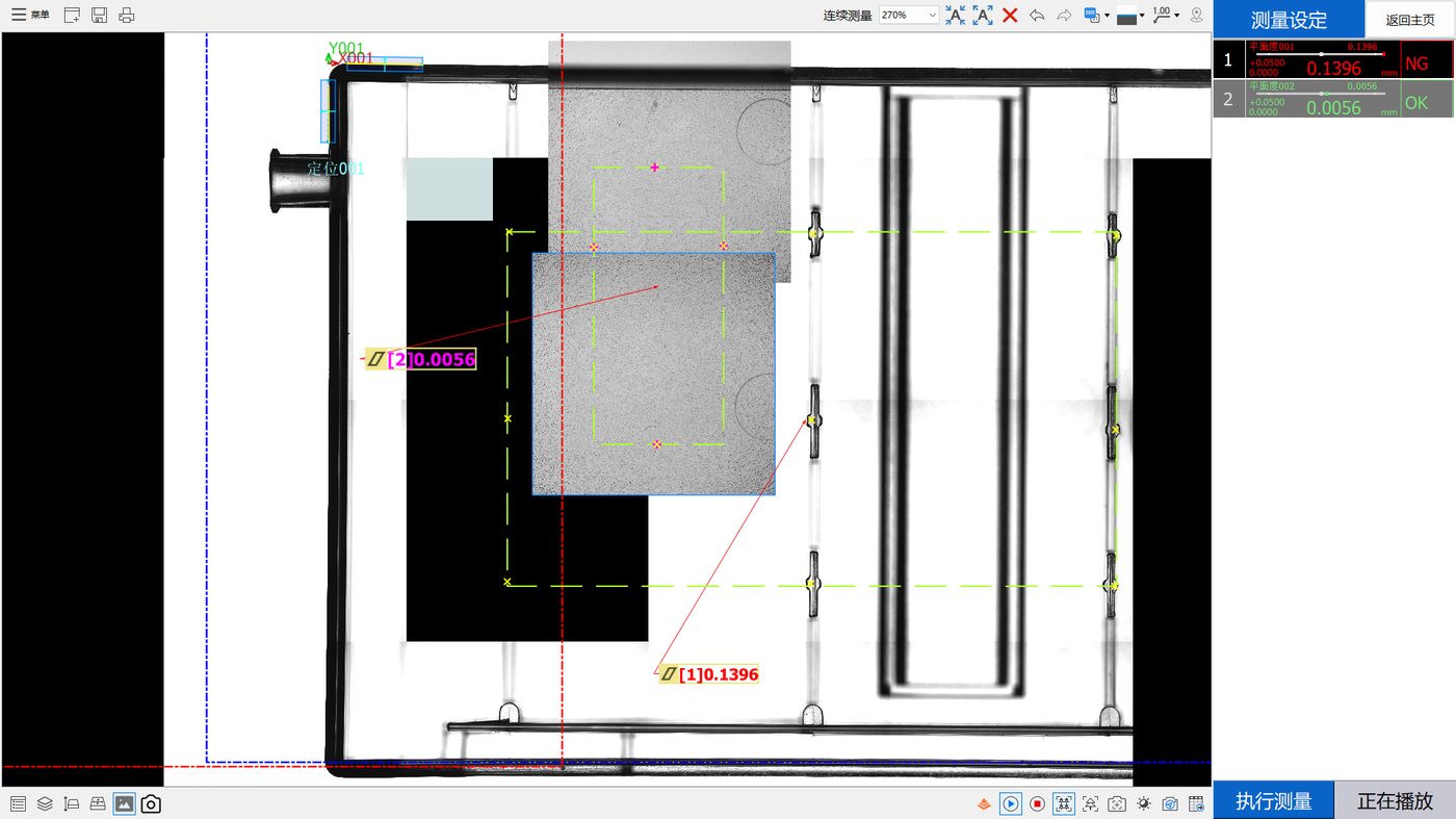
The structure of the data, first
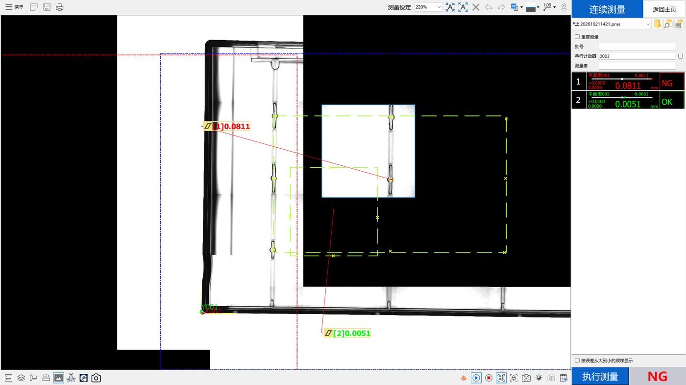
The data comes from one evaluation run on each of two parts, left and right. Two independent flatness zones were defined inside each measurement program, labelled zone 001 and zone 002, and each part was measured six times.
One clarification matters very early. A zone is not a point. In the statistics region of the file, each column is the result for a zone, not the reading at a location; in the detail region, each timestamp carries the values produced that cycle for each zone. So this data supports a discussion about differences between zones, but it does not support reconstruction down to "this specific point moved this much". That ceiling governs everything below.
How large is the discrepancy
The table below gives the mean, range and verdict for all four zone results, in millimetres, taken verbatim from the statistics region.
| Run | Zone | Mean | Range | OK / NG | Cpk |
|---|---|---|---|---|---|
| Right | Zone 001 | 0.1403 | 0.0088 | 0 / 6 | -9.532584 |
| Right | Zone 002 | 0.0060 | 0.0017 | 6 / 0 | 24.949094 |
| Left | Zone 001 | 0.0852 | 0.006 | 0 / 6 | -2.784232 |
| Left | Zone 002 | 0.0045 | 0.0014 | 6 / 0 | 33.262189 |
All four zones share the same upper specification limit of 0.05 mm and identical scoring logic. Against that single consistent rule, zone 001 fails six times out of six on both parts, and zone 002 passes six times out of six on both.
Reading note: the Cpk values above were computed by the software from these six samples. They characterise this sample set only and must not be read as long-term process capability or converted into a production yield.
Why the verdicts diverge
Because the zones were never on the same scale to begin with
Different areas of a moulded part deform for different reasons and by different amounts. Areas near the gate, transitions in wall thickness, large unsupported spans, and faces intended to seal against another component do not shrink or warp in the same way. Rolling all of them into one evaluation average hides the differences: a genuinely failing local area can be diluted into compliance, and a local feature can be amplified into a whole-part failure.
Because the choice of fitting rule changes the answer
A flatness result depends on which points are taken and how the reference plane is fitted through them. Minimum zone, least squares and other approaches return different numbers for the same point set. When a part has clearly separated functional areas, splitting it into planes with explicit functional meaning usually resolves more disputes than arguing about fitting algorithms ever will.
Because this is not a stability problem
To judge whether a measurement is stable, look at the spread between repeated readings on the same zone. In this data, zone 001 ranges 0.0088 mm on the right part and 0.006 mm on the left - small relative to its own mean. Zone 002 is tighter still. The readings converge, which means the setup returns consistent answers for the same area.
What changes is the difference between areas. That is a property of the workpiece, not jitter in the measurement. Separating those two things is what makes the conversation productive.
When you should split into multiple zones
Decide from function, not from aesthetics of the drawing. The following cases usually require independent zones.
| Case | Why it must be split |
|---|---|
| The face seals, bonds or clamps against another part | Local voids affect function directly; a global average cannot stand in for local behaviour |
| The area contains a wall thickness transition or ribs | Shrinkage differs from adjacent areas; one combined zone masks both |
| The part has both cosmetic and mating surfaces | Their requirements do not share a single basis and should not share one verdict |
| Deformation is directional, such as unidirectional bow | Directionality must be quantified per area; a single value discards that information |
| A downstream operation reshapes this area again | The local datum has to be locked at this step to avoid error accumulation |
The opposite holds too. If the surface really is one continuous, uniform plane with no functional subdivision and no mating relationship, describing it with one zone is correct. Splitting it further only adds subjectivity and cost.
Turning the conclusion into a scheme
Four steps, in order. First, sit down with product and process engineers and map the functional zones onto the surface; the output should be an annotated drawing, not a paragraph of prose. Second, define sampling method and density per zone - density should track the area and the width of its tolerance band, not be uniform everywhere. Third, fix the fitting rule and the verdict basis for each zone and write them into the measurement program. Fourth, validate the scheme with repeated measurements and check that scatter within each zone is acceptable.
Once those four steps are done, magnitude differences between zones stop being something to argue about and become structured results that manufacturing, quality and product engineering can all use.
Frequently asked questions
A twentyfold difference - is one of the values simply wrong?
Nothing in this data suggests an error. The six readings within a single zone converge; zone 001 on the right part spans only 0.0088 mm. The readings are self-consistent. What differs is the magnitude across areas, which is a part characteristic rather than measurement noise. To exclude equipment influence properly, standard artefacts would need to be run on the same setup.
Can we quote the passing zone and ignore the failing one?
No. The zones were split precisely because different areas do different jobs and deform by different amounts. Letting a good area cancel a bad one defeats the purpose of evaluating them separately. The correct move is to establish what each area must deliver and then issue separate verdicts and dispositions.
Is more zones always better?
No. Zones should be function-driven, not count-driven. Over-splitting shrinks the sample behind each fit, raises subjectivity, makes reports harder to read and complicates lot-to-lot comparison. A sensible granularity is one zone per functional area.
When should the fitting rule be decided?
At the time the measurement program is built, and it should be frozen in documentation alongside the requirement. Deciding the fitting rule later, after a dispute arises, removes the traceability value of everything already measured.
Does the data tell us which location is raised?
It does not. The file provides zone-level results only, with no point-level detail. Obtaining spatial distribution means retaining per-point records in the measurement scheme, or running a dedicated sampling routine over the area.
What is the very next action?
Confirm the physical area behind each zone and its functional role in the product, with product, process and quality in the room. After that, establish whether the excess in the failing area can be attributed to a specific moulding or assembly step. Only then revisit sampling and fitting.
Related reading
Full background of the underlying data is in the case article; the response sequence after divergent verdicts is in the troubleshooting article; and the interpretation of aggregate indicators such as NG rate is covered separately.
Related products and configuration notes
- POMEAS MX Automatic Vision Measuring Machine - Multi-sensor platform suited to running several independently scored zones on one part
- POMEAS IMAGE 3 Instant Vision Measuring System - Documents up to 300 features measured simultaneously, useful when one program must cover many areas
- SFS-D606 compact chromatic confocal sensor - 20 mm diameter body, about 73 g; positioned for sensor arrays and coplanarity or step measurement
Related reading
- Transparent Plastic Part Flatness Inspection: What Two Data Sets Actually Show
- Flatness Out of Tolerance: A Troubleshooting Path That Actually Works
- What Flatness Really Means, and What It Is Often Confused With
- Flatness Measurement Methods Compared: Plate, CMM, Vision, Confocal
- Repeatability Is Not Accuracy: Reading Range, Sigma and Cpk Honestly
- How to Choose Flatness Inspection Equipment: A Five-Step Reverse Method
- Point Spectral Confocal for Transparent Plastics: Benefits, Limits and Four Mistakes
- Multi-Point or Single-Point Flatness: Choosing How to Collect the Points
- Where Warpage in Injection Moulded Parts Comes From
- Turning Inspection Data into Decisions: Four Stages of Refinement
Related POMEAS product categories
The hardware referred to above is grouped into the following categories on the product side, with the specifications and model list for each range.
- 3D White Light Interferometer / Optical Surface Profiler — 3D white light interferometer profilers for roughness, step height and flatness.

Subscribe to Our Newsletter
Simply enter your email to receive the latest news and insights from Pomeas. Stay connected with Pomeas and be the first to discover new innovations in optical excellence.