Knowledge
Transparent Plastic Part Flatness Inspection: What Two Data Sets Actually Show
Flatness is one of those geometric tolerances that everyone assumes they understand until a report lands on the table and nobody agrees on what the number means. The reason is structural: flatness is not read off a scale. It is a derived quantity. You collect a set of points on the surface, fit an ideal plane through them under some rule, and only then get a number.
Change any link in that chain and the number changes. Below is a real inspection data set from a customer sample evaluation, reproduced without embellishment. Every figure in this article traces back to the two raw files that the measurement software exported. We do not beautify the result, and we do not speak for the equipment.
The problem this measurement was asked to solve
The workpiece is a transparent plastic structural part, supplied as a left and a right component, and it has to be confirmed before assembly. The difficulty is not whether it can be photographed. It is three things at once.
First, the material transmits light. A contact probe risks deforming a relatively compliant surface, and conventional imaging struggles to lock onto an edge when the background shows through. Second, several distinct zones on the part need evaluation, and they do not share a single height datum. Third, what the shop floor needs is a repeatable criterion, not a one-off description of what somebody saw that morning.
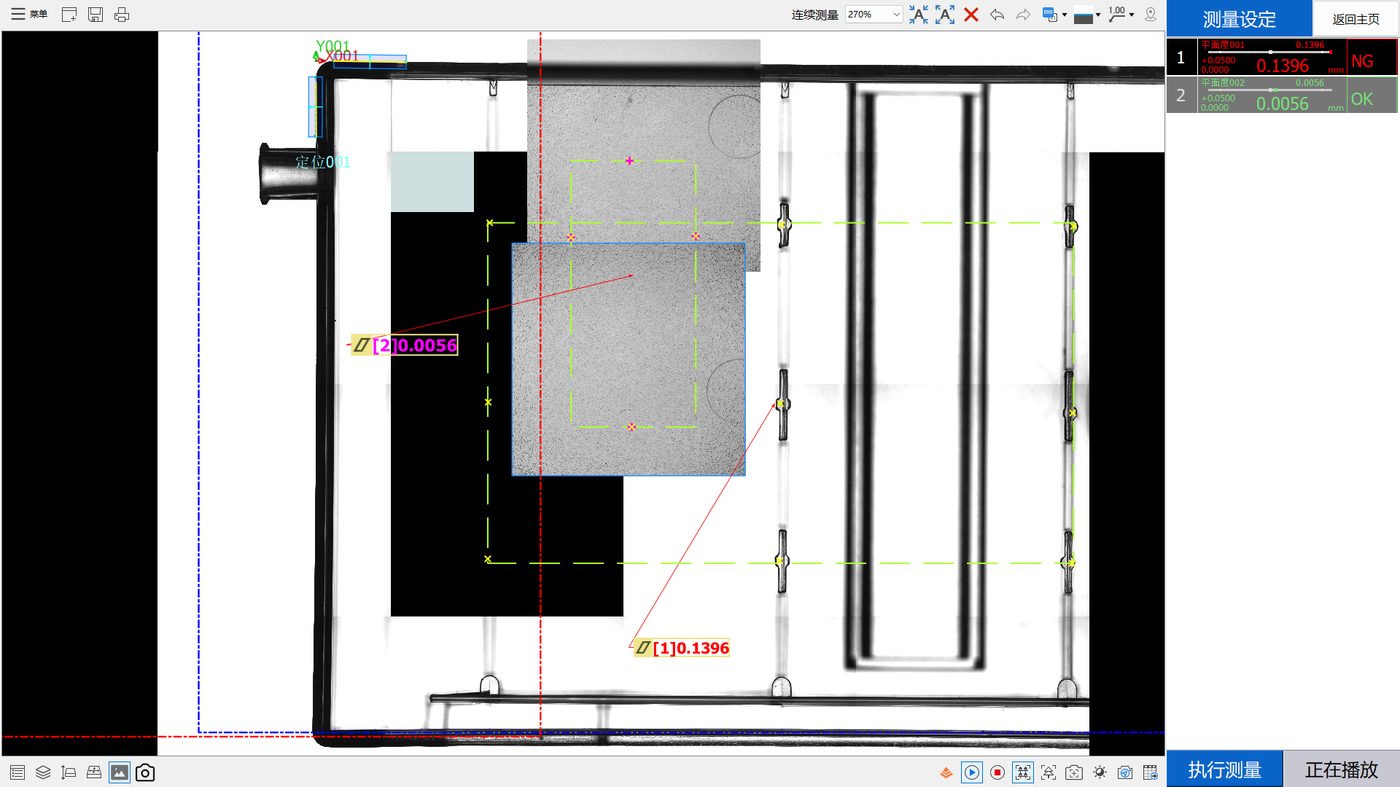
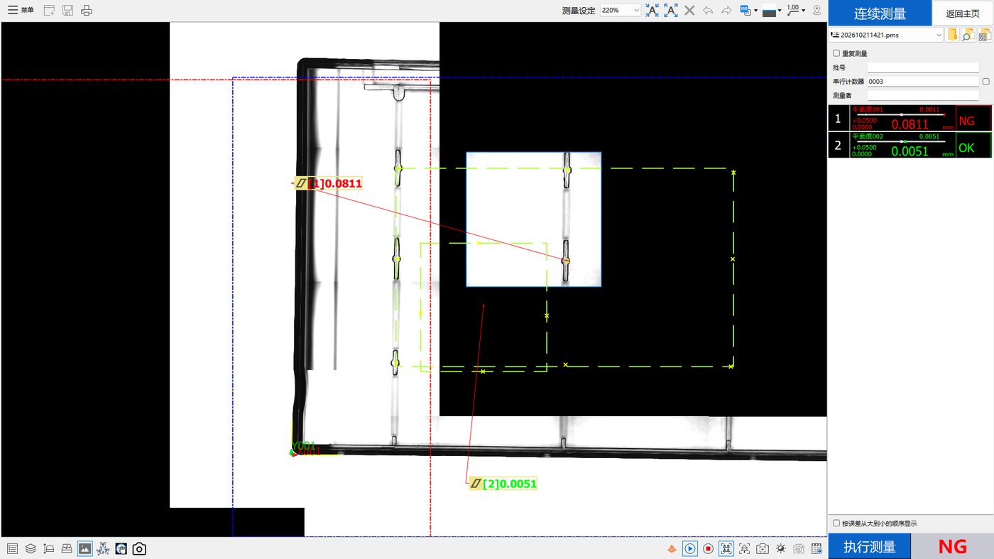
Under those constraints the evaluation was set up with non-contact optical sampling, with two independent flatness zones defined inside one measurement program so that different areas of the part could be scored separately. Each part was then measured six times so the spread of the readings could be observed under a single clamping condition.
What is actually inside the data table
The exported table has two regions. The upper region holds summary statistics; the lower region holds the individual records. Understanding that split is the entry ticket for reading any inspection report.
The statistics region: one run summarised
The statistics region is laid out by evaluation zone. For each zone it reports the number of valid measurements, the OK and NG counts and the NG rate, the design value, the upper and lower specification limits, maximum and minimum, mean, range, standard deviation and multiples of it, plus Cp and Cpk. Each column corresponds to an evaluation zone, not to a physical point.
The detail region: every individual reading
The detail region records each cycle chronologically: timestamp, the pass/fail verdict the software issued, a sequence number, and the reading produced for each zone that cycle. Every statistic above is computed from these raw values. So when a statistic looks odd, the fastest check is always to go back to the detail region.
The measured data
Two parts, each with its own program, six valid measurements each. All values below are taken verbatim from the statistics region. Units are millimetres.
| Statistic | Right, zone 001 | Right, zone 002 | Left, zone 001 | Left, zone 002 |
|---|---|---|---|---|
| Valid measurements | 6 | 6 | 6 | 6 |
| OK / NG | 0 / 6 | 6 / 0 | 0 / 6 | 6 / 0 |
| Upper specification limit | 0.0500 | 0.0500 | 0.05 | 0.05 |
| Maximum | 0.1447 | 0.0069 | 0.0891 | 0.005 |
| Minimum | 0.1359 | 0.0052 | 0.0831 | 0.0036 |
| Mean | 0.1403 | 0.0060 | 0.0852 | 0.0045 |
| Range (max - min) | 0.0088 | 0.0017 | 0.006 | 0.0014 |
| Standard deviation | 0.003156 | 0.000588 | 0.004022 | 0.000456 |
| Cpk | -9.532584 | 24.949094 | -2.784232 | 33.262189 |
| Software verdict | NG | OK | NG | OK |
The two files were exported with different decimal formatting - the right-hand file uses four fixed decimals, the left-hand file uses the native output precision. We reproduce both verbatim rather than padding or rounding, because normalising the text would change what was recorded.
Three things worth taking away
One: two zones on the same part, two opposite verdicts
Zone 001 on the right part averages 0.1403 mm and fails all six cycles. Zone 002 on the same part averages 0.0060 mm and passes all six. The left part behaves identically in kind: 0.0852 mm against 0.0045 mm. The gap is more than twentyfold on the right part and close to nineteenfold on the left.
The practical lesson is this: under one clamping, in one program, different areas of a single part can deform to completely different magnitudes. Treating one probe location as representative of "the flatness of this part" is not a simplification, it is a category error. The question worth asking is which zones need independent scoring, and what band each one should carry.
Two: the failures are not all the same kind
Zone 001 produces negative Cpk values (-9.532584 on the right part, -2.784232 on the left). That happens because the mean already sits beyond the 0.05 mm upper limit, so the numerator in the Cpk expression goes negative and the arithmetic returns a negative value. This is the formula behaving normally. It is not a software fault and it is not a measurement failure.
Equally, it does not mean anything beyond that. Negative Cpk says the mean of this sample sits outside the current limit. It cannot be converted into an accuracy figure, and it cannot be written down as the customer's acceptance verdict. We deal with that distinction separately below.
Three: how tight is the spread really
For zone 001 the range is 0.0088 mm on the right part and 0.006 mm on the left. Zone 002 is an order of magnitude tighter. Range and standard deviation describe scatter, which is to say they answer one specific question: given the same conditions, does this setup return the same number again?
They do not answer whether that number is right. Excellent scatter can sit comfortably around a wrong central value. Conversely, a scattered set of readings does not automatically indict the system; part settling, thermal drift and clamping relaxation all leave their fingerprints here. Keeping these two questions apart is the precondition for reading any measurement report honestly.
What this data supports, and what it does not
Stating the boundary plainly matters more than stacking up conclusions. The table below separates what may be written from what may not, so nothing gets repeated into a claim the data cannot carry.
| Supported by the data | Not supported by the data |
|---|---|
| The six individual readings for each run, with their ranges and standard deviations | An equipment accuracy figure derived from these readings |
| Scatter within each zone across those six cycles | A performance claim such as "this model achieves X" |
| The OK/NG verdict issued against the configured 0.05 mm limit | The customer's final acceptance decision |
| The large magnitude gap between the two zones on one part | Long-term process capability, production Cpk or yield |
| Where each zone mean sits relative to the configured limit | Point-by-point flatness distribution across the surface |
On Cp and Cpk: the values in this table were computed automatically by the software from six samples. They describe that small sample set and nothing more. They are not a statement of long-term process capability, which would require many lots, far more samples and stable production conditions.
Equipment accuracy is not in this table, and for a reason: twelve readings cannot establish it. That figure comes from the configuration itself, and for the integrated point-spectral confocal flash measurement setup used here, measurement accuracy reaches 2 μm. Keep the two apart when quoting this case - the numbers above describe these parts, the 2 μm figure describes the equipment.
What to do next
Faced with one zone failing and one passing, the order of operations matters. Establish which physical area each zone actually covers, and what that area does in the assembly. Then go to the moulding and assembly process and decide whether the excess originates in tooling, cooling, ejection or downstream assembly stress. Only then adjust the measurement approach itself: zone boundaries, sampling density, the fitting rule and the fixturing.
In that chain, the measurement scheme is the thing you eventually freeze, but it comes last. Define the object first. Until you do, you have a number that generates argument rather than a number that drives improvement.
Frequently asked questions
What exactly is the 0.05 mm figure in this data?
It is the upper specification limit for flatness configured inside the measurement program at the time these runs were produced. All four evaluation zones across both files carry the same value, and the software issues its OK or NG verdict against it. If any other tolerance needs to appear alongside it, engineering must first confirm that the two share the same basis. This article does not infer agreement between figures it has not verified.
Why does the same part produce NG and OK at the same time?
Because the two zones address different areas of the part and are sampled, fitted and scored independently. The data shows the two zone means differing by more than a factor of twenty on the right-hand part. That is not an instrument error; it is a demonstration that overall flatness on this part cannot be described with a single value.
Are six measurements enough?
Six repeats are enough to see whether readings converge under fixed conditions. They are nowhere near enough to characterise a process. Cp and Cpk only carry meaning over large samples, so at n = 6 they should be read as what they are - arithmetic applied to a small sample - and not as a verdict on process capability.
Does a negative Cpk mean the measurement failed?
No. When the zone mean sits outside the upper specification limit, the term representing distance from the mean to the nearest limit becomes negative and the result follows. It flags the position of the mean relative to the limit. It is not a fault indication, and it is not equivalent to any acceptance decision.
Is flatness on transparent parts measured differently from opaque ones?
The difference is mainly in how points are acquired. Contact probes risk deforming compliant transparent plastics, and ordinary 2D imaging has trouble holding an edge when light passes through the material. Non-contact optical sampling with deliberate illumination is therefore the usual route. Whether a given scheme works depends on transmission, surface condition and geometry, and should be confirmed with actual samples.
Can this data be used to state a yield figure?
No. Yield and long-term capability require samples across lots and shifts under stable production conditions. This data covers one day, one part type, two pieces and six cycles each. Its purpose is to show whether the measurement scheme is serviceable and whether the zone split is sensible, not to extrapolate yield.
Related reading
For the geometry and definitions behind zone evaluation see the companion article on two zones returning opposite verdicts; for the response sequence after a failure see the troubleshooting path article; for the measurement concepts see the article on why repeatability is not accuracy.
Related products and configuration notes
- POMEAS MX Automatic Vision Measuring Machine - Multi-sensor platform documented for 2D/3D dimensions, form tolerance, cross-section profiles, height difference and thickness
- POMEAS IMAGE 3 Instant Vision Measuring System - Up to 300 features and 100 targets in a single program; documented operating environment 20 +/- 1 C
- SFS-D410 chromatic confocal displacement sensor - 10 mm reference distance, +/- 0.2 mm measuring range; 12 nm repeatability per official specification
- 20 kHz multi-channel confocal controller - Supports 4 / 8 / 12 / 16 sensor heads for synchronised multi-point acquisition
Related reading
- Two Flatness Zones, Two Opposite Verdicts on the Same Part
- Flatness Out of Tolerance: A Troubleshooting Path That Actually Works
- What Flatness Really Means, and What It Is Often Confused With
- Flatness Measurement Methods Compared: Plate, CMM, Vision, Confocal
- Repeatability Is Not Accuracy: Reading Range, Sigma and Cpk Honestly
- How to Choose Flatness Inspection Equipment: A Five-Step Reverse Method
- Point Spectral Confocal for Transparent Plastics: Benefits, Limits and Four Mistakes
- Multi-Point or Single-Point Flatness: Choosing How to Collect the Points
- Where Warpage in Injection Moulded Parts Comes From
- Turning Inspection Data into Decisions: Four Stages of Refinement
Related POMEAS product categories
The hardware referred to above is grouped into the following categories on the product side, with the specifications and model list for each range.
- 3D White Light Interferometer / Optical Surface Profiler — 3D white light interferometer profilers for roughness, step height and flatness.

Subscribe to Our Newsletter
Simply enter your email to receive the latest news and insights from Pomeas. Stay connected with Pomeas and be the first to discover new innovations in optical excellence.