Knowledge
Industrial Zoom Lens for Laboratory Applications: What a Bench Setup Needs
A laboratory bench rarely inspects the same part twice in the same way, and that single fact decides most of the optical specification. Unlike a production line, where one magnification is calibrated once and repeated all shift, a lab handles samples of different sizes in the same session, documents what it sees, and often hands the images to someone who was not at the bench. A manual industrial zoom lens paired with an industrial camera fits that pattern better than any fixed-magnification instrument, because the operator changes magnification continuously and the record is a file, not a memory. This article sets out what a laboratory configuration needs: a zoom range matched to the sample set, sampling that matches the smallest feature, a working distance that matches the stand, and a record that can be compared months later.
What a laboratory bench asks from the optics
Three tasks dominate bench work. The first is observation: looking at a sample until the operator understands its structure, which demands a wide magnification range and forgiving depth of field. The second is documentation: saving frames that show a feature with enough context that a colleague can interpret them without the sample in hand. The third is comparison: coming back weeks later, setting the same magnification, and checking whether anything changed. Each task taxes a different part of the system. Observation taxes the zoom range, documentation taxes resolution and illumination, and comparison taxes repeatability and record-keeping. A bench that only optimises one of the three produces sharp images that nobody can reproduce.
The laboratory also differs from the production line in who uses the image. On a line, the judgement is automated and the optics only need to satisfy a recipe. At a bench, a person interprets the frame, so contrast and even illumination matter as much as resolution, and the operator will happily trade the last micrometre of resolution for a field that keeps the whole feature visible with its surroundings.
Why the manual zoom is the laboratory default
A manual continuous zoom lens changes magnification by turning a dial, with no motor, no controller and no software in the loop. For a bench operator that is the fastest possible interface: the hand moves from sample to dial and back in the same motion, and magnification follows attention in real time. The POMEAS manual families cover the ranges a laboratory actually uses. The 12.5× family spans 0.58× to 7.5×, which on a 2/3-inch sensor means a field from 15.17 × 11.38 mm down to 1.17 × 0.88 mm. The 6.5× family spans 0.7× to 4.5× for samples that live in the middle of that range, and the 4K series reaches 0.68× to 5.0× on a 1-inch sensor with an 18.8 mm wide field at the bottom end.
The case for a motorized lens appears only when magnification must be reproduced exactly, under software control, every time. That is a production requirement. In a laboratory, the operator judges focus and framing by eye anyway, so a motor adds cost without removing the human from the loop — with the exception of laboratories that record the magnification value for every frame, which is a documentation habit rather than an optics requirement.
Size the range from the sample set, not from the dial
The published 12.5× table shows what one family covers on a 2/3-inch sensor:
| Magnification | FOV (H × V) | Depth of field | Object-side resolution |
|---|---|---|---|
| 0.58× | 15.17 × 11.38 mm | 2.75 mm | 13 µm |
| 1.0× | 8.80 × 6.60 mm | 0.95 mm | 7.8 µm |
| 2.0× | 4.40 × 3.30 mm | 0.27 mm | 4.53 µm |
| 3.0× | 2.93 × 2.20 mm | 0.15 mm | 3.73 µm |
| 4.5× | 1.96 × 1.47 mm | 0.081 mm | 3.05 µm |
| 7.5× | 1.17 × 0.88 mm | 0.056 mm | 3.05 µm |
Two rules fall straight out of the table. First, the widest sample that must fit in one frame sets the minimum magnification: a 14 mm circuit board region needs about 0.6×, which is why the low end matters as much as the high end. Second, the smallest feature the lab must see sets the useful maximum, and the limit arrives earlier than most people expect. Object-side resolution stops improving at 3.05 µm from 4.5× upward, because the numerical aperture has reached 0.11 and stays there. Beyond that point the field simply gets smaller; the detail does not get finer.
Sampling: what the camera contributes
Object-side resolution is the optics’ ceiling, but the recorded image is limited by the coarser of the two: the optics or the sensor sampling. Sampling in micrometres per pixel is the field width divided by the horizontal pixel count. With a 1920-pixel-wide frame, the same table gives 7.9 µm/px at 0.58×, 2.3 µm/px at 2.0× and about 0.6 µm/px at 7.5×. A feature is reliably visible only when it spans enough pixels and has contrast, which is why a 13 µm optical resolution at 0.58× is paired with 7.9 µm per pixel — the sensor, not the lens, is the binding limit at the bottom of the range. The practical consequence for a laboratory is to buy the camera after the magnification table, not before: a sensor with very small pixels does not add detail at low magnification, and at high magnification the optics stop improving at 3.05 µm regardless of the sensor behind them.
Working distance and the stand
Working distance is set by the stand as much as by the lens, and in a laboratory it competes with access: probes, tweezers or a soldering tip may need to reach the sample while it is in view. The POMEAS 6.5× family is specified at 87 ± 2 mm with the 12 mm fine-focus variant, which leaves genuine tool access; the same family also exists with a 3 mm fine-focus travel for benches that never need tools under the lens. The 12.5× family works closer, which is acceptable for observation-only benches. The stand should carry the fine focus rather than the lens barrel: depth of field at 4.5× is 0.081 mm, and a coarse stand knob cannot reliably position inside that window. These trade-offs mirror the ones at a repair bench, and the same arithmetic applies.
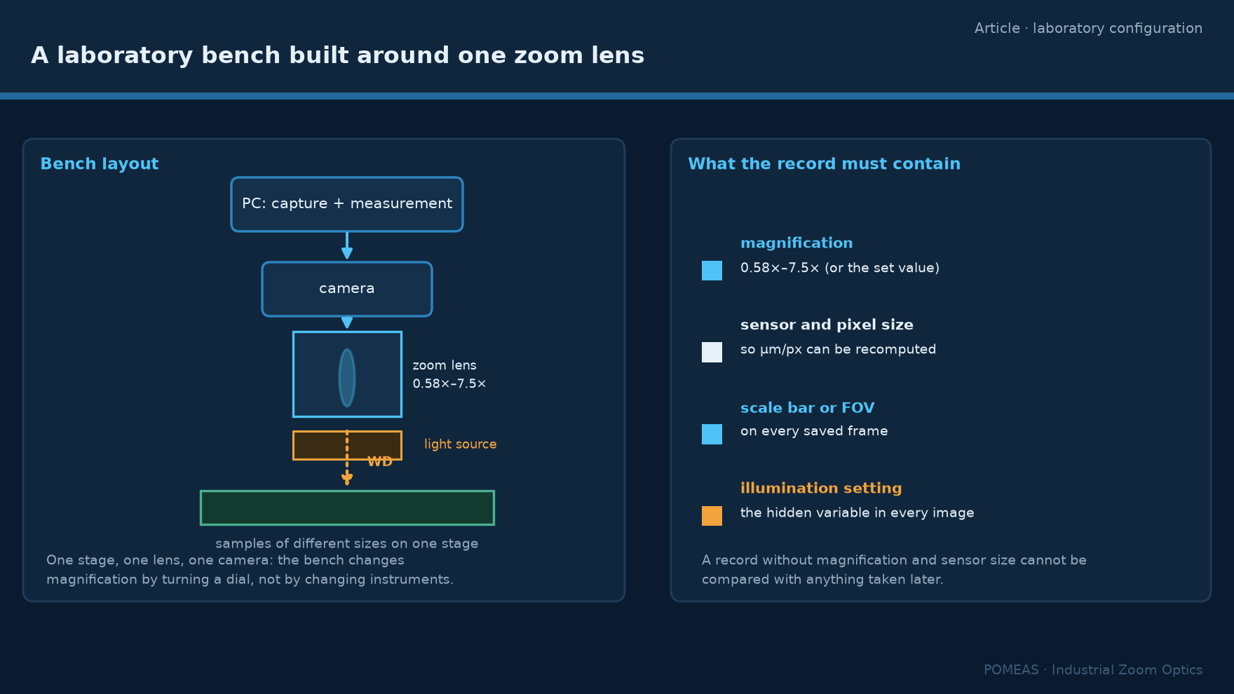
The record: what every saved frame must carry
A laboratory image is data only if it can be interpreted later. Four values make a frame reproducible: the magnification, the sensor and its pixel size, a scale bar or the field of view, and the illumination setting. Magnification and sensor size together let anyone recompute micrometres per pixel and compare the frame with any other frame taken on the bench. Illumination is the hidden variable — two frames at the same magnification with different illumination angles can look like different samples. None of this requires software beyond a capture utility; it requires a habit, applied every time. Laboratories that skip it accumulate images that are sharp, beautiful and scientifically unusable.
Two laboratory configurations that cover most cases
Configuration one, the observation and documentation bench: a PMS-LZL-12101D 12.5× manual zoom lens with coaxial illumination on a stand with fine focus, a 2/3-inch camera, and a capture utility that stamps magnification into the file name or metadata. This covers samples from a full connector to a bond wire and records what it sees. Configuration two, the materials bench with occasional near-limit work: the same zoom body with an APO objective chain for the highest-magnification sessions, which trades working distance and field for resolution the zoom alone cannot reach. The modular path and its boundary conditions are described in the digital microscope build guide. Both configurations are deliberately built from standard components, because a laboratory’s needs change faster than an integrated instrument can be re-specified.
For samples that are transparent or reflective, configuration choices change again: coaxial illumination and polarization become primary decisions rather than accessories. The transparent-surface setup guide covers that case separately.
Frequently asked questions
Can one zoom lens really cover a whole PCB and a 0.2 mm component?
Yes, if the range is chosen from the sample set. The 12.5× family spans fields from 15.17 mm wide at 0.58× to 1.17 mm at 7.5× on a 2/3-inch sensor, which covers a board region down to a bond wire. What changes across that range is depth of field, from 2.75 mm to 0.056 mm, so stage focus becomes more critical as magnification rises.
Does a laboratory need a motorized zoom lens?
Only if magnification must be reproduced exactly under software control, which is a production and repeatability requirement. At a bench where a person judges focus and framing, a manual zoom is faster to use and simpler to maintain, and the magnification value can still be recorded for every frame.
Why does my image go out of focus when I zoom in?
Depth of field shrinks as magnification rises — from 2.75 mm at 0.58× to 0.056 mm at 7.5× in the published table — so the same stage position that was sharp at low magnification sits outside the focus window at high magnification. Parfocal design keeps the shift small, but a fine focus adjustment is still expected at each end of the range.
What camera should I pair with a laboratory zoom lens?
Choose the camera after the magnification table. At 1920 px width the sampling is 7.9 µm/px at 0.58× and about 0.6 µm/px at 7.5×; the optics themselves stop improving past 3.05 µm above 4.5×. A sensor far smaller than those numbers adds no detail, so spend the budget on illumination and a good stand instead.
Can APO objectives be added to a zoom lens later?
Yes, on zoom bodies designed to take objective chains. The zoom provides the framing range and the APO objective raises numerical aperture for the finest features, at the cost of working distance and field. The combination is a standard laboratory architecture, and the selection checklist for zoom-plus-objective systems walks through the compatibility checks.
What must an image record contain to be usable later?
Magnification, sensor and pixel size, a scale bar or field of view, and the illumination setting. With those four values anyone can recompute micrometres per pixel and compare the frame against later work. Without them the image is anecdotal, however sharp it looks.

Subscribe to Our Newsletter
Simply enter your email to receive the latest news and insights from Pomeas. Stay connected with Pomeas and be the first to discover new innovations in optical excellence.