Knowledge
Build a Multi-Magnification Machine Vision Inspection System
A multi-magnification system lets one camera do two jobs that normally need two stations: find and locate at low magnification, then judge detail at high magnification. There are three architectures that achieve this, and they fail in different ways. Choosing between them is a decision about cycle time, fixture tolerance and calibration, not about optics alone. This article sets out the three options, the arithmetic that separates them, and the six steps that turn the choice into a working system.
Three architectures, three failure modes
One zoom lens, several recipe magnifications. The lens stays mounted, the zoom group moves, and the recipe records which magnification each step uses. Failure mode: depth of field changes by a factor of tens across the range, so a part that is in focus at low magnification may not be at high magnification.
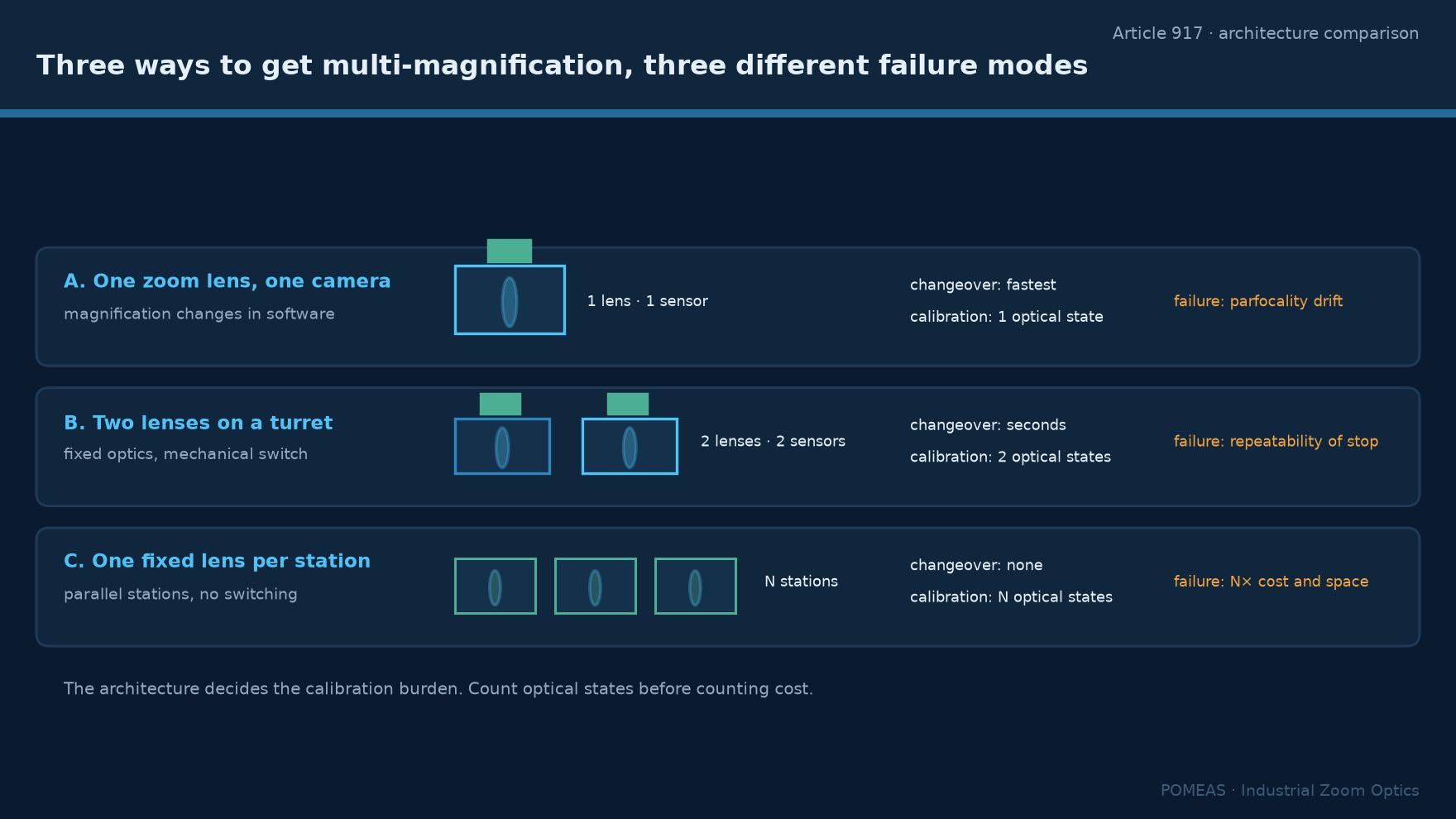
Several fixed lenses on a turret or a linear slide. Each magnification has its own optics, so each is optimised. Failure mode: parcentricity. Swapping lenses moves the optical axis, so the target that was centred at 1× is off-centre at 5×, and the stage has to re-find it.
Two or more stations, each with one magnification. The part moves between stations. Failure mode: throughput and part handling, plus the cost of a second camera and a second motion axis.
Most production systems choose the first option, because it preserves centring and removes handling, and then pay for it with focus management. The comparison between a single zoom and a fixed lens at one magnification is covered in zoom lens versus fixed focal lens.
The range arithmetic, using real published data
The POMEAS 12.5× motorised lens PMS-LZL-12104-D1 covers 0.58× to 7.5× at 77.4 ± 2 mm working distance on a 2/3-inch sensor. Its published table gives the numbers below. Fields are object-side, width × height.
| Magnification | FOV on 2/3″ | DOF | NA | Resolution |
|---|---|---|---|---|
| 0.58× | 15.17 × 11.38 mm | 2.75 mm | 0.025 | 13 µm |
| 1.0× | 8.80 × 6.60 mm | 0.95 mm | 0.043 | 7.8 µm |
| 1.5× | 5.87 × 4.40 mm | 0.43 mm | 0.063 | 5.3 µm |
| 2.0× | 4.40 × 3.30 mm | 0.27 mm | 0.074 | 4.53 µm |
| 3.0× | 2.93 × 2.20 mm | 0.15 mm | 0.09 | 3.73 µm |
| 4.5× | 1.96 × 1.47 mm | 0.081 mm | 0.11 | 3.05 µm |
| 6.0× | 1.47 × 1.10 mm | 0.061 mm | 0.11 | 3.05 µm |
| 7.5× | 1.17 × 0.88 mm | 0.056 mm | 0.11 | 3.05 µm |
Two features of that table drive system design. Depth of field falls by a factor of 49 from the low end to the high end, while resolution improves by only a factor of 4.3. The high-magnification end therefore demands a flat, well-supported part and buys a modest optical gain; the low end is where the tolerance is easy and the information content is low.
Step 1: decide which magnification carries the measurement
Only one magnification should carry a dimensional decision. Pick it by the smallest feature that must be judged, then check that the field at that magnification still contains the feature plus its reference edges. If it does not, the system needs stitching at that magnification, which changes the timing budget substantially.
At 7.5× the field is 1.17 mm wide, which contains a 0.5 mm die with margin but not a 2 mm package. At 3× the field is 2.93 mm, which contains the package but resolves only 3.73 µm. This is the trade that cannot be avoided, and the way out is to measure at 3× with a sub-pixel edge algorithm rather than to measure at 7.5× and stitch.
Step 2: treat focus as a per-magnification problem
Because depth of field at 6× is 0.061 mm and at 0.58× is 2.75 mm, a system that switches magnification must also verify focus at the new setting, or accept a defocused image. Three options exist: a focus axis that moves the camera or the lens, a lens with a fine-focus ring driven by a second motor, and a fixture that holds the part flat enough that a single focus position works at all magnifications. The third is cheapest and is the one most often skipped.
Where a focusing axis exists, the search range can be bounded by the expected part height variation rather than by the full travel, which keeps the focus step short. The relationship between working distance, depth of field and focus error is set out in how to improve depth of field in industrial zoom lenses.
Step 3: count the time honestly
The cycle time of a multi-magnification recipe is not the sum of exposure times. It is the sum of, per magnification: zoom move and settle, focus search, illumination settle, exposure, and image transfer. A zoom move that takes 300 ms and a focus search that takes 400 ms will dominate a 20 ms exposure by more than an order of magnitude. Two practical consequences: keep the number of magnification changes per part as low as the inspection plan allows, and order the steps so that all features at one magnification are measured before switching.
This is where the field-count arithmetic from a large-part inspection pays off: if a 600 mm part needs 1,156 fields at a 20 mm field, the number of magnification changes matters far less than the number of moves, and the opposite is true for a small part inspected at two magnifications in a single field.
Step 4: check parcentricity if you ever change hardware
With one lens, centring is preserved across magnifications only within the lens's own parcentricity specification. With multiple lenses or a turret, it is not preserved at all. Either way, the system needs a calibration that maps image coordinates to stage coordinates at each magnification, and that calibration has to be repeated whenever a lens, camera or mount changes. The procedure for verifying that a lens change did not move the axis is described in replacing a C-mount lens on an existing vision cell.
Step 5: verify that magnification is repeatable, not just present
A motorised zoom lens returns to a commanded position, but "position" and "magnification" are related by a curve that has backlash, hysteresis and temperature dependence. If the recipe assumes that pulse position 4200 always means 3.00×, a repeatability test is required to confirm the assumption. The test method, including cycle count and acceptance criterion, is described in motorised zoom lens repeatability. For a multi-magnification system, the test should be run at each magnification the recipe uses, not only at one.
Step 6: choose detented or continuous on purpose
A detented lens gives defined, identifiable magnification steps; a continuous lens gives any value in range but no repeatable reference. For a recipe with two or three fixed magnifications, detents are easier to validate and easier to document. For a system that must scan magnification to find a feature, continuous is necessary. The difference is explained in what is detent magnification, and the control interface that reports position back to the PLC is described in motorised zoom lens RS-232 protocol.
What a multi-magnification system does not fix
It does not extend the optical resolution limit: below about 3 µm, a zoom lens in this class stops improving no matter how far it is zoomed. It does not remove the need for a flat part at high magnification. It does not make a low-contrast feature visible: if the defect is a transparent layer on a reflective surface, changing magnification will not create contrast that the illumination does not provide. And it does not replace a telecentric system for dimensional measurement, because a zoom lens has neither a constant magnification across the field nor a calibrated scale.
Frequently asked questions
How many magnifications should a recipe use?
As few as the inspection plan allows, usually two: one to locate and one to judge. Each additional magnification adds a zoom move, a focus search and a calibration reference to the cycle, and the time cost is usually larger than the optical benefit.
Can I use one zoom lens for both 0.5× overview and 7× detail?
Yes, within one lens family. The POMEAS 12.5× motorised lens covers 0.58× to 7.5× in one optical path, which means the part stays centred and no handling is required. The cost is that depth of field at 7.5× is 0.056 mm, so the part must be flat or supported.
Why does my image shift when the lens changes magnification?
Because no zoom lens is perfectly parcentric: the optical axis moves slightly as the groups travel. The shift is specified per lens and is usually a fraction of a percent of the field. A recipe that returns to the same coordinates after a zoom change should either allow a re-find step or use a lens with a tight parcentricity specification.
Is it cheaper to use two fixed lenses than one motorised zoom?
On hardware cost, often yes. On system cost, not necessarily: two lenses need a turret or a second camera, a parcentricity calibration and either handling or a second station, and those items frequently exceed the price difference. The decision should be made on total cost including calibration and floor space.
What camera resolution suits a multi-magnification recipe?
Size it for the highest magnification that carries a measurement. At 7.5× the field is 1.17 mm wide, so a 1920-pixel camera samples 0.61 µm per pixel, which is already finer than the 3.05 µm optical resolution. A larger sensor crops the field at the same magnification, which may be an advantage at low magnification and a limitation at high.
Do I need a separate illumination setting per magnification?
Yes. The illuminated area shrinks with the field, so a ring light optimised for a 15 mm field will overexpose a 1.2 mm field. Most systems store illumination level with the magnification in the recipe, and coaxial illumination is usually reserved for the high-magnification step.

Subscribe to Our Newsletter
Simply enter your email to receive the latest news and insights from Pomeas. Stay connected with Pomeas and be the first to discover new innovations in optical excellence.