Knowledge
FPC Ribbon Inspection: Resolving 10 µm Defects Across a 5.5 mm Field
A system-level selection guide for inline inspection of touch-panel FPC ribbons: full-width coverage in one field of view, with credible sampling of 10 µm-class defects. All field-of-view and pixel-sampling figures are theoretical calculations, pending sample-based verification.
Project Background: The Microscope Sees It, But the Line Can't Keep Up
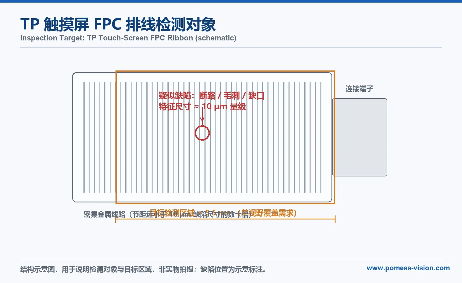
In FPC (flexible printed circuit) inspection the same trade-off appears everywhere: the microscope resolves the defect, but cannot keep pace with production.
An operator at a microscope can spot 10 µm-class trace anomalies — opens, notches, burrs, scratches. But the field of view is only a millimetre or so across, so a ribbon several centimetres long must be stepped through section by section: inspection falls behind takt time and miss rates climb with fatigue. Switch to a wide-field standard FA lens and the problem inverts — the field is there, but 10 µm defects sink into the noise floor. Closing that gap is what telecentric optics, plus deliberate camera and lighting selection, is for.
Note: this article is written around a stated target condition of a ~5.5 mm ribbon width and ~10 µm target defect size. The actual product model, defect catalogue and acceptance criteria remain subject to the customer's process documentation (see the pending-confirmation list in the review package).
Why FPC Inspection Is Hard
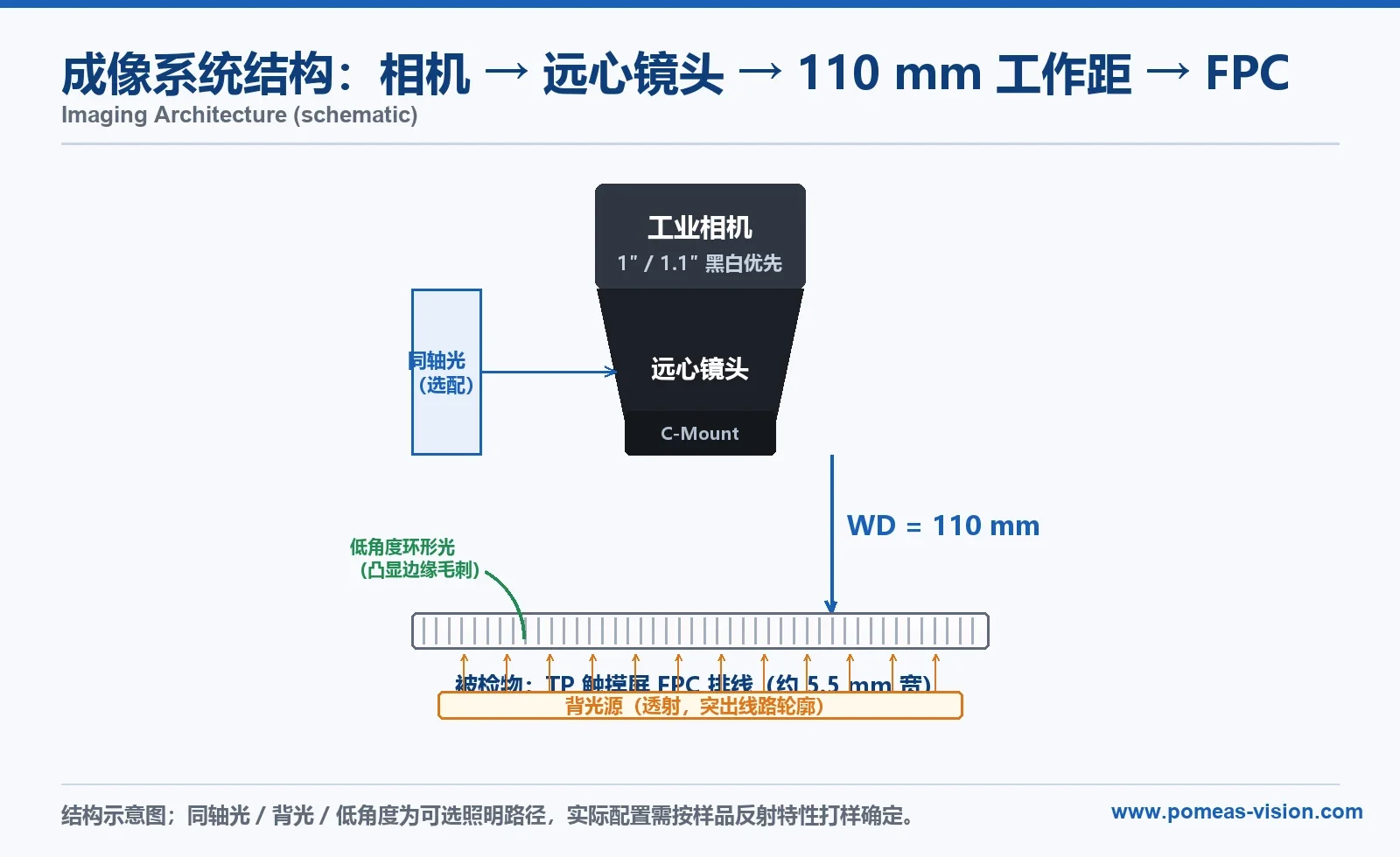
1. Wide field vs. fine detail. A 5.5 mm ribbon examined for ~10 µm features spans a 1:550 ratio. A 5 MP sensor covering it yields ~2.2 µm per pixel, but conventional lenses lose resolution and gain distortion toward the field edges, smearing exactly the features that matter.
2. Specular, densely packed traces. Metal traces mirror-reflect and repeat every few tens of microns; under plain diffuse lighting, defect contrast washes out.
3. Thin, warping parts. FPC is typically ~0.1 mm thick and bows after handling; the optics need depth-of-field headroom to hold focus across the field.
4. Manual inspection leaves no data. Step-by-step visual checks are slow, inconsistent, and disconnected from MES/SPC loops.
POMEAS Imaging Configuration
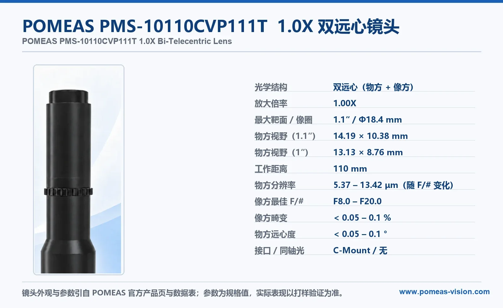
Three decisions drive the optical design: the lens structure (telecentric), the sensor match (field of view and pixel sampling), and the lighting (contrast).
2.0X High-Resolution Telecentric Lens Options
Within POMEAS's current 2.0X telecentric range, the highest-resolution options are the PMS-LTCM2-110 and its coaxial-illuminated counterpart, the LTCM2-110C:
| Parameter | PMS-LTCM2-110 | LTCM2-110C |
|---|---|---|
| Magnification | 2.0X | 2.0X |
| Working distance | 110 mm | 110 mm |
| Object-side resolution | 4.53 µm | — (NA 0.0074) |
| Depth of field (theoretical) | 0.27 mm | 0.27 mm (Φ0.04 mm CoC) |
| F-number | 13.5 | 13.5 |
| TV distortion | 0.03% | 0.03% |
| Max. sensor format | 2/3″ | 2/3″ (≤5 MP) |
| Field of view (2/3″) | 4.4 × 3.3 mm | 4.4 × 3.3 mm |
| Coaxial illumination | No | Optional |
| Mount | C-Mount | C-Mount |
The conclusion is blunt: at 2.0X on a 2/3″ sensor the field is only 4.4 × 3.3 mm — narrower than the ribbon. A single-field 2.0X solution would require a 1.1″-format 2.0X telecentric lens.
For reference, the customer's current 2.0X + 1.1″ setup uses the VWK20-110-111 / VWK20-110C-111 — WWK-series object-side telecentric lenses from Shenzhen NEW TRY (Langce), not POMEAS models. Quoted from the manufacturer's datasheet purely as a comparison point: 2.0X, WD 110 ± 2 mm, up to Φ18.0 mm (1.1″) image circle, best F/# 13.5, MTF30 > 60 lp/mm, DoF ± 0.2 mm at F20, distortion < 0.1%, telecentricity < 0.1°, object field ≈ 7.1 × 5.2 mm on 1.1″ (the -C variant adds coaxial illumination). It covers the ribbon, but with limited margin.
1.0X Bi-Telecentric Lens: The Recommended Path
For single-field coverage of the ribbon with measurement-grade, double-telecentric imaging inside the POMEAS catalogue, the recommended lens is the PMS-10110CVP111T:
| Parameter | PMS-10110CVP111T |
|---|---|
| Optical structure | Bi-telecentric (object- and image-side) |
| Magnification | 1.00X |
| Max. sensor format | 1.1″ / Φ18.4 mm |
| Object field of view (1.1″) | 14.19 × 10.3 mm (per product page) |
| Working distance | 110.00 mm |
| Depth of field | 0.66–1.60 mm |
| Image-side best F/# | 8.00–20.00 |
| Image-side MTF30 | 120–50 lp/mm |
| Object-side resolution | 5.37–13.42 µm |
| Object-side telecentricity | <0.05–0.1° |
| Distortion | <0.05–0.1% |
| Total length / O-I distance | 132.88 mm / 260.41 ± 2 mm |
| Mount / coaxial | C-Mount / non-coaxial |
| Operating temperature | 0–60 °C |
Why this lens — and what it costs:
- Ample single-field coverage. The object field is 14.19 × 10.3 mm on a 1.1″ sensor; the ribbon occupies about 39% of it, leaving generous alignment tolerance.
- Bi-telecentric stability. Magnification does not change with small axial part movement, and distortion stays below 0.05–0.1%, which keeps defect coordinates stable and calibration honest.
- The trade-off is coarser sampling. At 1.0X a 10 µm defect spans fewer pixels than at 2.0X (below); a larger sensor recovers part of that cost.
- If coaxial light is required at 1.0X: the PMS-LTCM1-110C (1.0X, 110 mm WD, 7.46 µm object-side resolution, DoF 0.89 mm, F11, coaxial) is an alternative — with different sensor-format and resolution specs, the FOV math must be redone against the chosen camera.
1-Inch Industrial Camera Options
Once the lens format is fixed, the camera determines pixel sampling. Compatible POMEAS cameras (all C-mount):
| Model | Format | Resolution | Pixel | Frame rate | Interface / shutter | Mono/Color |
|---|---|---|---|---|---|---|
| PMS-CCN120VP2ABSC | 1.1″ | 4096 × 3072 (12.6 MP) | 3.4 µm | 9.4 fps | GigE / global shutter | Mono |
| PMS208CCUA1C | 1″ | 5480 × 3648 (20 MP) | 2.4 µm | 22 fps | USB3.0 / rolling shutter | Color |
| PMSCCN2008VPH2 | 1″ | 5480 × 3648 (21 MP) | — | — | GigE (PoE) / hardware trigger | Color |
Recommendation: for defect inspection prefer monochrome + global shutter — no Bayer interpolation, no motion artefacts. If finer sampling is the priority, the 1″ 20 MP camera offers 2.4 µm pixels at the cost of a rolling shutter, acceptable only for static or slow-moving conditions.
Field of View and Pixel-Sampling Calculations
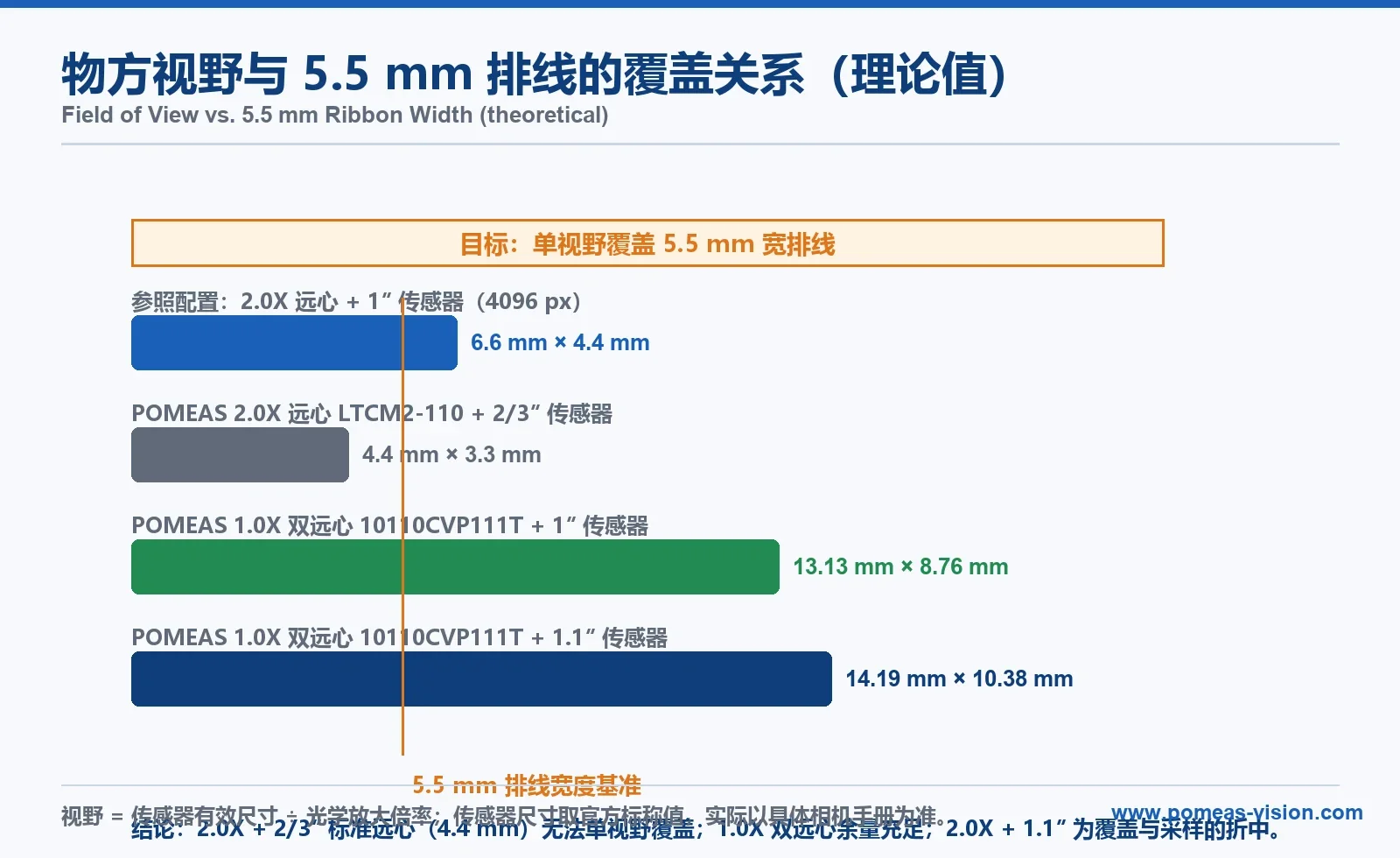
All figures below are theoretical calculations framing the configuration envelope — not demonstrated capability.
① Object field of view = sensor active area ÷ magnification
| Configuration | Object FOV | Covers 5.5 mm ribbon in one field? |
|---|---|---|
| 2.0X + 2/3″ (LTCM2 series) | 4.4 × 3.3 mm | ✕ No |
| 2.0X + 1.1″ (customer's VWK-class setup) | ≈7.1 × 5.2 mm | ✓ (limited margin) |
| 1.0X + 1″ (PMS-10110CVP111T) | 13.13 × 8.76 mm | ✓ |
| 1.0X + 1.1″ (PMS-10110CVP111T) | 14.19 × 10.3 mm | ✓ (ample margin) |
② Object-side pixel scale = pixel pitch ÷ magnification
| Configuration | Pixel scale | Sampling of a 10 µm defect |
|---|---|---|
| 2.0X + 1.1″, 4096 px (3.4 µm pixels) | 1.70 µm/px | ≈ 5.9 px |
| 1.0X + 1″, 5480 px (2.4 µm pixels) | 2.40 µm/px | ≈ 4.2 px |
| 1.0X + 1.1″, 4096 px (3.4 µm pixels) | 3.40 µm/px | ≈ 2.9 px |
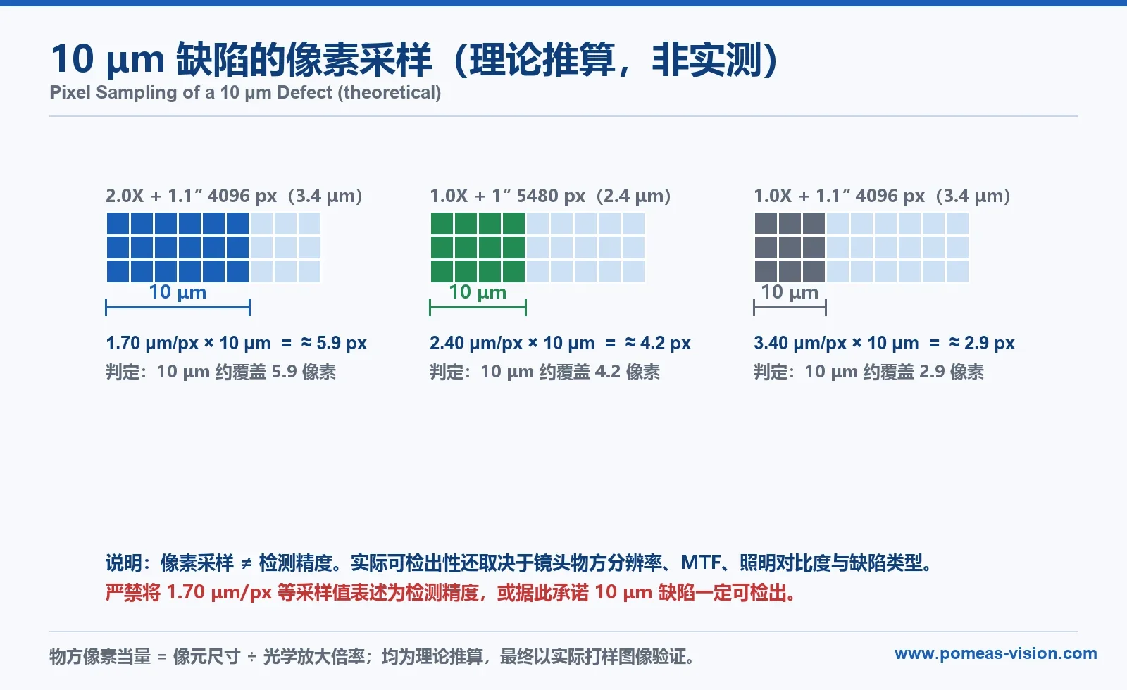
③ The critical reading — pixel sampling is not detection accuracy
Three points must be stated plainly:
- A pixel scale of 1.70 µm/px must never be presented as "1.70 µm detection accuracy," nor as a guarantee that 10 µm defects will be found.
- Take the PMS-LTCM2-110 as an example: its specified object-side resolution is 4.53 µm, while a 2.0X setup on a 3.4 µm-pixel camera samples at just 1.70 µm/px — the pixels are already finer than the lens's resolving power. The real bottleneck is the lens's optical resolution, its MTF, and illumination contrast — not the pixel count. High magnification is not high resolution (see Magnification Is Not Resolution).
- The PMS-10110CVP111T's specified object-side resolution spans 5.37–13.42 µm depending on F/#. A 10 µm feature sits inside that band — on the boundary between resolvable and not. Only sample-based verification with real parts can settle it; this article makes no guarantee either way.
Choosing the Right Illumination
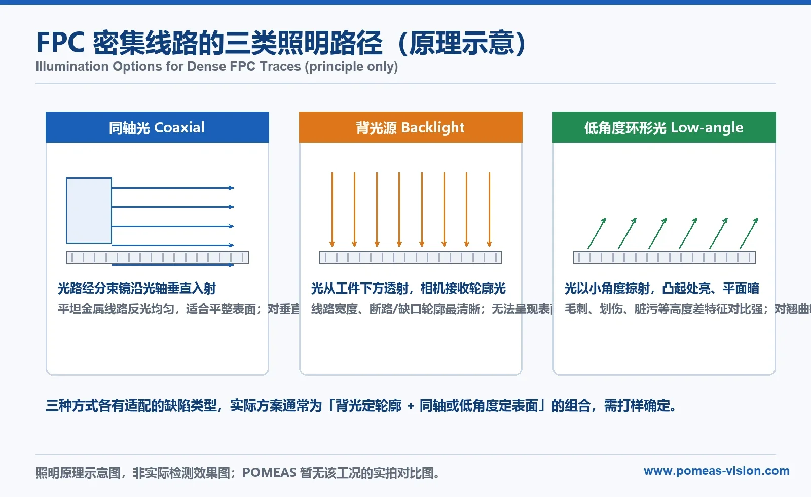
On dense metal traces, lighting decides half the image quality. Three paths, mapped to defect types (the figures in the full package are principle diagrams, not inspection results):
| Lighting | Optical behaviour | Best suited for |
|---|---|---|
| Coaxial | Light folded onto the optical axis; specular reflection returns uniformly | Overall imaging of flat metal traces, surface contamination; weak on vertical steps and burrs |
| Backlight | Transmitted from below; camera sees silhouette | Trace width, opens, notches — sharpest for contour defects; no surface relief |
| Low-angle | Glancing light; raised features bright, flats dark | Burrs, scratches, contamination (height-difference features); warp-sensitive |
Practical notes:
- Contour defects (opens/shorts/notches): start with backlight; with a telecentric lens it gives crisp silhouettes.
- Surface defects (scratches, dents, stains): A/B coaxial vs. low-angle on real samples.
- Coaxial requires the right lens: the LTCM2-110C supports optional coaxial illumination; the recommended PMS-10110CVP111T is non-coaxial, so if coaxial proves necessary the combination must be re-confirmed with POMEAS engineering (pending item).
From Calculation to Sample Verification
Theory can only prove the configuration is not over-stretched; actual detection must be verified on hardware:
- FOV and magnification survey — real object field, magnification error and distortion map on a calibration target.
- Resolution check — USAF target or real traces at the working F/#, to see which end of the 5.37–13.42 µm band the system delivers.
- Defect-sample runs — customer samples or known rejects, verified class by class under candidate lighting; record the smallest detectable feature per class.
- Warp tolerance — focus held across the full field at the worst expected part bow.
- Takt time — acquisition plus processing against target throughput.
Acceptance thresholds belong to the customer's process owner; the supplier provides data support. Define criteria first, then verify — not the reverse.
From Static Capture to Inline Production
Once samples pass, the move to production adds:
- Triggering — encoder or PLC hardware triggers; the part stationary or uniformly moving during exposure.
- Registration — Mark-point or fixture referencing aligns the inspection ROI to the ribbon coordinates.
- Decision logic — template matching and edge differencing for contour defects; a rule-based screen plus AI classifier for surface defects, thresholds calibrated from sample data.
- Data loop — defects logged by web coordinate for MES/SPC, tracing back to the process station.
- Environment — check the lens operating range (0–60 °C) against line conditions.
Object-Side Pixel Equivalent: The Formula Behind Every Sampling Check
Every "can this lens resolve a 10 µm defect" question reduces to a single number — the object-side pixel equivalent: how much workpiece distance one camera pixel covers.
Object-side pixel equivalent (µm/px) = sensor pixel size (µm) ÷ optical magnification (×)
It is not field of view divided by pixel count. That shortcut agrees only when the magnification is itself derived from the same field of view; used on its own it hides the sensor-to-lens mismatch that produces under-sampled images.
| Configuration | Sensor pixel size | Optical magnification | Object-side pixel equivalent | Pixels across a 10 µm feature |
|---|---|---|---|---|
| 1-inch, 5480 px sensor | 2.4 µm | 1.0X | 2.40 µm/px | ≈ 4.2 px |
| 1.1-inch, 4096 px sensor | 3.4 µm | 1.0X | 3.40 µm/px | ≈ 2.9 px |
| 1.1-inch, 4096 px sensor | 3.4 µm | 2.0X | 1.70 µm/px | ≈ 5.9 px |
Every figure above is theoretical arithmetic, not a measured detection result. The same 5.5 mm ribbon leaves 2.9 px per 10 µm feature with a 3.4 µm sensor at 1.0X, and 5.9 px at 2.0X — the camera did not change, the magnification did.
Three checks before locking a configuration
- Coverage — object field of view = sensor width (µm) ÷ magnification. A 4096 × 3.4 µm sensor at 1.0X spans ≈ 13.9 mm, enough for a 5.5 mm ribbon with margin; the same sensor at 2.0X spans only ≈ 7.0 mm.
- Sampling — the object-side pixel equivalent must leave enough pixels across the smallest feature you must see. More pixels are not automatically better: doubling magnification halves the field of view.
- Physical limit — pixel count is not optical resolution. Lens object-side resolution and illumination contrast set the floor, and only a sampling test on real parts confirms what is actually detectable.
Related reading: Magnification Is Not Resolution, 1.1-Inch Camera and Telecentric Lens Matching, Object-Side Resolution vs Measurement Accuracy.
FAQ
Is the 1.70 µm pixel scale the same as 1.70 µm detection accuracy?
No. Pixel scale is only the sampling interval. Actual detectability depends on lens resolution, MTF, illumination contrast, defect type and algorithm, and is typically far coarser than the pixel scale — which is why every figure here is labelled theoretical.
Can the PMS-10110CVP111T guarantee detection of 10 µm defects?
No such guarantee can be made. Its specified object-side resolution of 5.37–13.42 µm places a 10 µm feature in the critical band; real detectability depends on the working F/#, illumination contrast and defect class, and must be verified by sampling.
Why not just use a 2.0X lens?
POMEAS's standard 2.0X telecentric lenses (LTCM2-110 / LTCM2-110C) top out at 2/3″ with a 4.4 × 3.3 mm field — too narrow for the ribbon. A single-field 2.0X solution would need a 1.1″-format 2.0X telecentric lens, absent from the current standard range.
Is a telecentric lens really necessary? Why not a standard FA lens?
Standard FA lenses introduce perspective, magnification drift with part-height variation, and higher edge distortion. Where stable coordinates and edge positions drive the judgement, double-telecentric optics is a clear advantage. See What Is a Telecentric Lens?.
Colour or monochrome camera?
Monochrome: no Bayer interpolation loss and stronger effective sampling; colour carries no decision value for metallic traces on polyimide in this condition.
Why 110 mm of working distance?
The 110 mm WD leaves room for fixtures, cover glass and lighting, and keeps the optics clear of bowing thin parts — a common working distance for FPC work.
POMEAS Machine Vision Optics
POMEAS supplies industrial lenses, cameras, lighting and measurement systems as one product line. For 10 µm-class FPC ribbon defect inspection, the recommended path is:
- Recommended: PMS-10110CVP111T (1.0X bi-telecentric, 1.1″) + a 1.1″ mono global-shutter camera (PMS-CCN120VP2ABSC) + lighting selected by sample trials per defect class.
- Alternatives: PMS-LTCM1-110C (1.0X coaxial) or LTCM2-110C (2.0X coaxial, multi-field stitching required).
- Customer's current reference: the 2.0X + 1.1″ VWK20-110 series (third-party model) — if retained, brand and supply considerations rest with the customer.
Further reading:
- Telecentric Lens Selection Guide
- Object-Side Resolution vs. Measurement Accuracy FAQ
- Camera Sensor and Lens Image Circle Matching
- Zoom Lens Selection for 10.4 mm FOV, 5 µm Defect Inspection
- Products: PMS-10110CVP111T 1.0X bi-telecentric lens | LTCM2-110 | LTCM2-110C
For a configuration review against a specific ribbon, contact POMEAS technical support with your camera model, target FOV, defect catalogue and installation envelope.

Subscribe to Our Newsletter
Simply enter your email to receive the latest news and insights from Pomeas. Stay connected with Pomeas and be the first to discover new innovations in optical excellence.